程序员实战，生成式对抗网络（GAN）下篇，tensorflow实现

一、程序代码

程序主要实现上篇文章中所提到的随机噪声拟合高斯分布的过程，话不多说，直接上代码：

#引入必要的包

import argparse

import numpy as np

from scipy.stats import norm

import tensorflow as tf

import matplotlib.pyplot as plt

import seaborn as sns

sns.set(color_codes=True)

#设置种子，用于随机初始化

seed =42

np.random.seed(seed)

tf.set_random_seed(seed)

#定义真实的数据分布，这里为高斯分布

classDataDistribution(object):

def __init__(self):

#高斯分布参数

#均值为4

self.mu =4

#标准差为0.5

self.sigma =0.5

def sample(self, N):

samples = np.random.normal(self.mu,self.sigma, N)

samples.sort()

return samples

#随机初始化一个分布，做为G网络的输入

classGeneratorDistribution(object):

def __init__(self, range):

self.range = range

def sample(self, N):

return np.linspace(-self.range,self.range, N)+ \

np.random.random(N)*0.01

#定义线性运算函数，其中参数output_dim=h_dim*2=8

def linear(input, output_dim, scope=None, stddev=1.0):

#定义一个随机初始化

norm = tf.random_normal_initializer(stddev=stddev)

#b初始化为0

const= tf.constant_initializer(0.0)

with tf.variable_scope(scope or'linear'):

#声明w的shape,输入为（12，1）*w，故w为（1，8），w的初始化方式为高斯初始化

w = tf.get_variable('w',[input.get_shape()[1], output_dim], initializer=norm)

#b初始化为常量

b = tf.get_variable('b',[output_dim], initializer=const)

#执行线性运算

return tf.matmul(input, w)+ b

#

def generator(input, h_dim):

h0 = tf.nn.softplus(linear(input, h_dim,'g0'))

h1 = linear(h0,1,'g1')

return h1

#初始化w和b的函数，其中h0,h1,h2,h3为层，将mlp_hidden_size=4传给h_dim

def discriminator(input, h_dim):

#linear 控制w和b的初始化,这里linear函数的第二个参数为4*2=8

#第一层

h0 = tf.tanh(linear(input, h_dim *2,'d0'))

#第二层输出，隐藏层神经元个数还是为8

h1 = tf.tanh(linear(h0, h_dim *2,'d1'))

#h2为第三层输出值

h2 = tf.tanh(linear(h1, h_dim *2, scope='d2'))

#最终的输出值

h3 = tf.sigmoid(linear(h2,1, scope='d3'))

return h3

#优化器 采用学习率衰减的方法

def optimizer(loss, var_list, initial_learning_rate):

decay =0.95

num_decay_steps =150

batch = tf.Variable(0)

#调用学习率衰减的函数

learning_rate = tf.train.exponential_decay(

initial_learning_rate,

batch,

num_decay_steps,

decay,

staircase=True

)

#梯度下降求解

optimizer = tf.train.GradientDescentOptimizer(learning_rate).minimize(

loss,

global_step=batch,

var_list=var_list

)

#返回

return optimizer

#构造模型

class GAN(object):

def __init__(self, data, gen, num_steps, batch_size, log_every):

self.data = data

self.gen = gen

self.num_steps = num_steps

self.batch_size = batch_size

self.log_every = log_every

#隐藏层神经元个数

self.mlp_hidden_size =4

#学习率

self.learning_rate =0.03

#通过placeholder格式来创造模型

self._create_model()

def _create_model(self):

#创建一个名叫D_pre的域，先构造一个D_pre网络，用来训练出真正D网络初始化网络所需要的参数

with tf.variable_scope('D_pre'):

#输入的shape为（12，1），一个batch一个batch的训练，

#每个batch的大小为12，要训练的数据为1维的点

self.pre_input = tf.placeholder(tf.float32, shape=(self.batch_size,1))

self.pre_labels = tf.placeholder(tf.float32, shape=(self.batch_size,1))

#调用discriminator来初始化w和b参数,其中self.mlp_hidden_size=4，为discriminator函数的第二个参数

D_pre = discriminator(self.pre_input,self.mlp_hidden_size)

#预测值和label之间的差异

self.pre_loss = tf.reduce_mean(tf.square(D_pre -self.pre_labels))

#定义优化器求解

self.pre_opt = optimizer(self.pre_loss,None,self.learning_rate)

# This defines the generator network - it takes samples from a noise

# distribution as input, and passes them through an MLP.

#真正的G网络

with tf.variable_scope('Gen'):

self.z = tf.placeholder(tf.float32, shape=(self.batch_size,1))

#生产网络只有两层

self.G = generator(self.z,self.mlp_hidden_size)

# The discriminator tries to tell the difference between samples from the

# true data distribution (self.x) and the generated samples (self.z).

#

# Here we create two copies of the discriminator network (that share parameters),

# as you cannot use the same network with different inputs in TensorFlow.

#D网络

with tf.variable_scope('Disc')as scope:

self.x = tf.placeholder(tf.float32, shape=(self.batch_size,1))

#构造D1网络，真实的数据

self.D1 = discriminator(self.x,self.mlp_hidden_size)

#重新使用一下变量，不用重新定义

scope.reuse_variables()

#D2，生成的数据

self.D2 = discriminator(self.G,self.mlp_hidden_size)

# Define the loss for discriminator and generator networks (see the original

# paper for details), and create optimizers for both

#定义判别网络损失函数

self.loss_d = tf.reduce_mean(-tf.log(self.D1)- tf.log(1-self.D2))

#定义生成网络损失函数

self.loss_g = tf.reduce_mean(-tf.log(self.D2))

self.d_pre_params = tf.get_collection(tf.GraphKeys.TRAINABLE_VARIABLES, scope='D_pre')

self.d_params = tf.get_collection(tf.GraphKeys.TRAINABLE_VARIABLES, scope='Disc')

self.g_params = tf.get_collection(tf.GraphKeys.TRAINABLE_VARIABLES, scope='Gan')

#优化，得到两组参数

self.opt_d = optimizer(self.loss_d,self.d_params,self.learning_rate)

self.opt_g = optimizer(self.loss_g,self.g_params,self.learning_rate)

def train(self):

with tf.Session()as session:

tf.global_variables_initializer().run()

# pretraining discriminator

#先训练D_pre网络

num_pretrain_steps =1000

for step in range(num_pretrain_steps):

#随机生成数据

d =(np.random.random(self.batch_size)-0.5)*10.0

labels = norm.pdf(d, loc=self.data.mu, scale=self.data.sigma)

pretrain_loss, _ = session.run([self.pre_loss,self.pre_opt],{

self.pre_input: np.reshape(d,(self.batch_size,1)),

self.pre_labels: np.reshape(labels,(self.batch_size,1))

})

#拿出预训练好的数据

self.weightsD = session.run(self.d_pre_params)

# copy weights from pre-training over to new D network

for i, v in enumerate(self.d_params):

session.run(v.assign(self.weightsD[i]))

#训练真正的网络

for step in range(self.num_steps):

# update discriminator

x =self.data.sample(self.batch_size)

#z是一个随机生成的噪音

z =self.gen.sample(self.batch_size)

#优化判别网络

loss_d, _ = session.run([self.loss_d,self.opt_d],{

self.x: np.reshape(x,(self.batch_size,1)),

self.z: np.reshape(z,(self.batch_size,1))

})

# update generator

#随机初始化

z =self.gen.sample(self.batch_size)

#迭代优化

loss_g, _ = session.run([self.loss_g,self.opt_g],{

self.z: np.reshape(z,(self.batch_size,1))

})

#打印

if step %self.log_every ==0:

print('{}: {}\t{}'.format(step, loss_d, loss_g))

#画图

if step %100==0or step==0or step ==self.num_steps -1:

self._plot_distributions(session)

def _samples(self, session, num_points=10000, num_bins=100):

xs = np.linspace(-self.gen.range,self.gen.range, num_points)

bins = np.linspace(-self.gen.range,self.gen.range, num_bins)

# data distribution

d =self.data.sample(num_points)

pd, _ = np.histogram(d, bins=bins, density=True)

# generated samples

zs = np.linspace(-self.gen.range,self.gen.range, num_points)

g = np.zeros((num_points,1))

for i in range(num_points // self.batch_size):

g[self.batch_size * i:self.batch_size *(i +1)]= session.run(self.G,{

self.z: np.reshape(

zs[self.batch_size * i:self.batch_size *(i +1)],

(self.batch_size,1)

)

})

pg, _ = np.histogram(g, bins=bins, density=True)

return pd, pg

def _plot_distributions(self, session):

pd, pg =self._samples(session)

p_x = np.linspace(-self.gen.range,self.gen.range, len(pd))

f, ax = plt.subplots(1)

ax.set_ylim(0,1)

plt.plot(p_x, pd, label='real data')

plt.plot(p_x, pg, label='generated data')

plt.title('1D Generative Adversarial Network')

plt.xlabel('Data values')

plt.ylabel('Probability density')

plt.legend()

plt.show()

def main(args):

model = GAN(

#定义真实数据的分布

DataDistribution(),

#创造一些噪音点，用来传入G函数

GeneratorDistribution(range=8),

#迭代次数

args.num_steps,

#一次迭代12个点的数据

args.batch_size,

#隔多少次打印当前loss

args.log_every,

)

model.train()

def parse_args():

parser = argparse.ArgumentParser()

parser.add_argument('--num-steps', type=int,default=3000,

help='the number of training steps to take')

parser.add_argument('--batch-size', type=int,default=12,

help='the batch size')

parser.add_argument('--log-every', type=int,default=10,

help='print loss after this many steps')

return parser.parse_args()

if __name__ =='__main__':

main(parse_args())

二、程序运行结果

1、程序运行初始状态

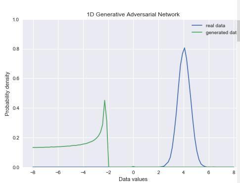
其中左边为随机初始化的数据，右边为真实的呈高斯分布的数据。

2、程序迭代运行1200次后的状态

这里不知道为什么原因，程序没有正常的拟合真实的数据，将迭代次数增加之后，程序也没有太大的变化，D和G网络的两个Loss的变化都很小，这里还望大家帮忙找一找原因。可能和GAN网络容易训练跑偏的一些原因有关。

留言，加入人工智能深度学习社群，跟小编一起讨论吧！